EP6: No Overlap, No Answer: The Positivity Assumption
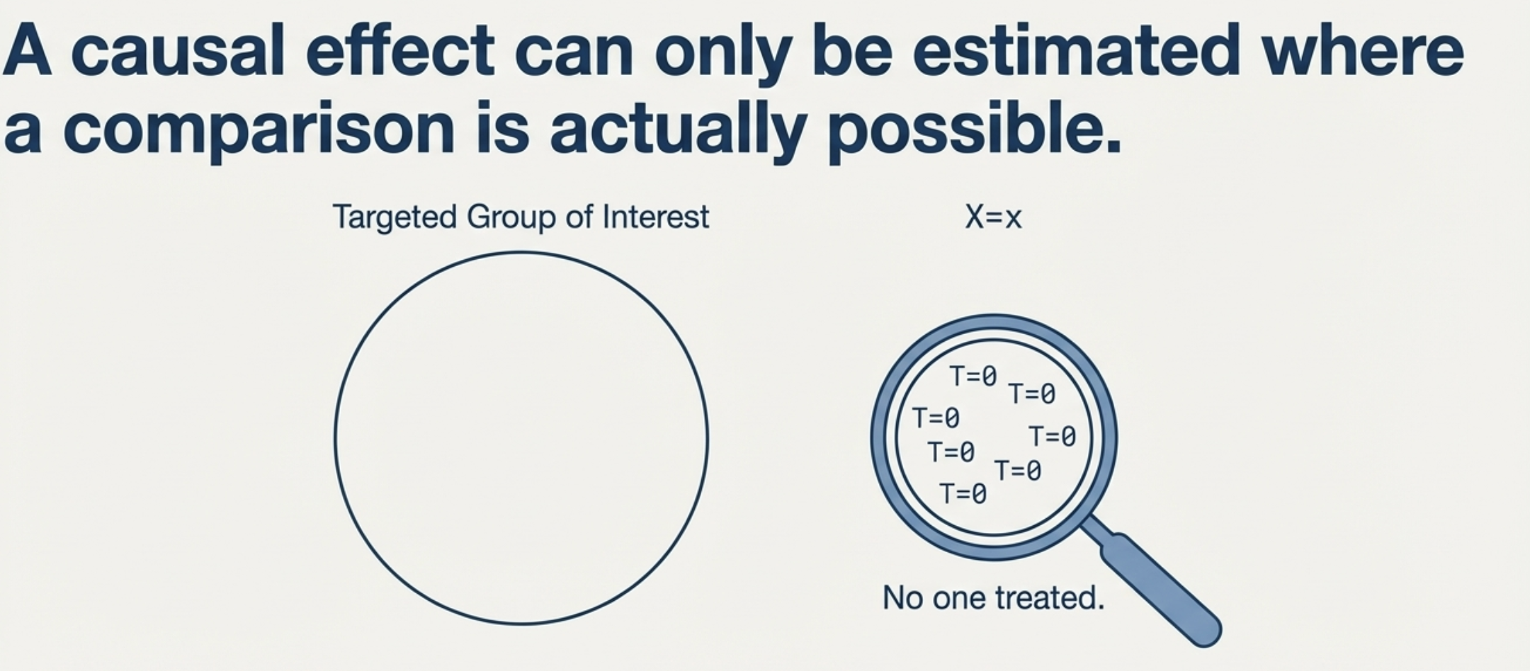
A causal effect can only be estimated where a comparison is actually possible.
Imagine you want to evaluate the impact of a loyalty programme on customer spend. You condition on customer segment, tenure, and region — adjusting for confounders so the treated and untreated groups are comparable (for more on this, see EP5).
But during your analysis, you discover a problem: for one particular segment—long-tenured enterprise customers—every single customer in your data is already enrolled in the programme. There are no unenrolled counterparts to compare against.
What is the effect of the programme for this specific group? You cannot say. There is no variation in treatment to learn from.
This is a violation of the Positivity Assumption. While exchangeability tells us the groups are comparable given covariates, positivity tells us the comparison must actually be possible in the first place.
Listen to This Episode
Want to dive deeper into the positivity assumption? This podcast episode provides more in-depth information and intuition. Tune in and follow the podcast to get notified when the next episode is out!
1. The Positivity Assumption: The Requirement for Overlap
In a randomized experiment, every unit has a real chance of landing in either group. The process that determines who gets treated — the assignment mechanism — is both unconfounded (that’s exchangeability) and probabilistic (Rubin 1990).
Positivity requires that this same probabilistic nature exists in our observational data. For every combination of covariates (\(X\)) present in our population, there must be a non-zero probability of receiving any level of treatment:
\[0 < P(T=1 \mid X=x) < 1 \quad \text{for all } x \text{ such that } P(X=x) > 0\]
This conditional probability is the propensity score, \(e(x) = P(T=1 \mid X=x)\).1 In our loyalty programme example: given a long-tenured enterprise customer, what is the probability they enrol? If the answer is 1 — everyone in that group enrols — there is no one left unenrolled to compare against, and the causal effect for that group is unidentifiable.2
Positivity is only required for the covariates \(X\) that are needed for exchangeability (Hernan and Robins 2024). In our example, segment, tenure, and region are the confounders you adjust for — positivity must hold for every combination of those three, but not for variables you don’t condition on.
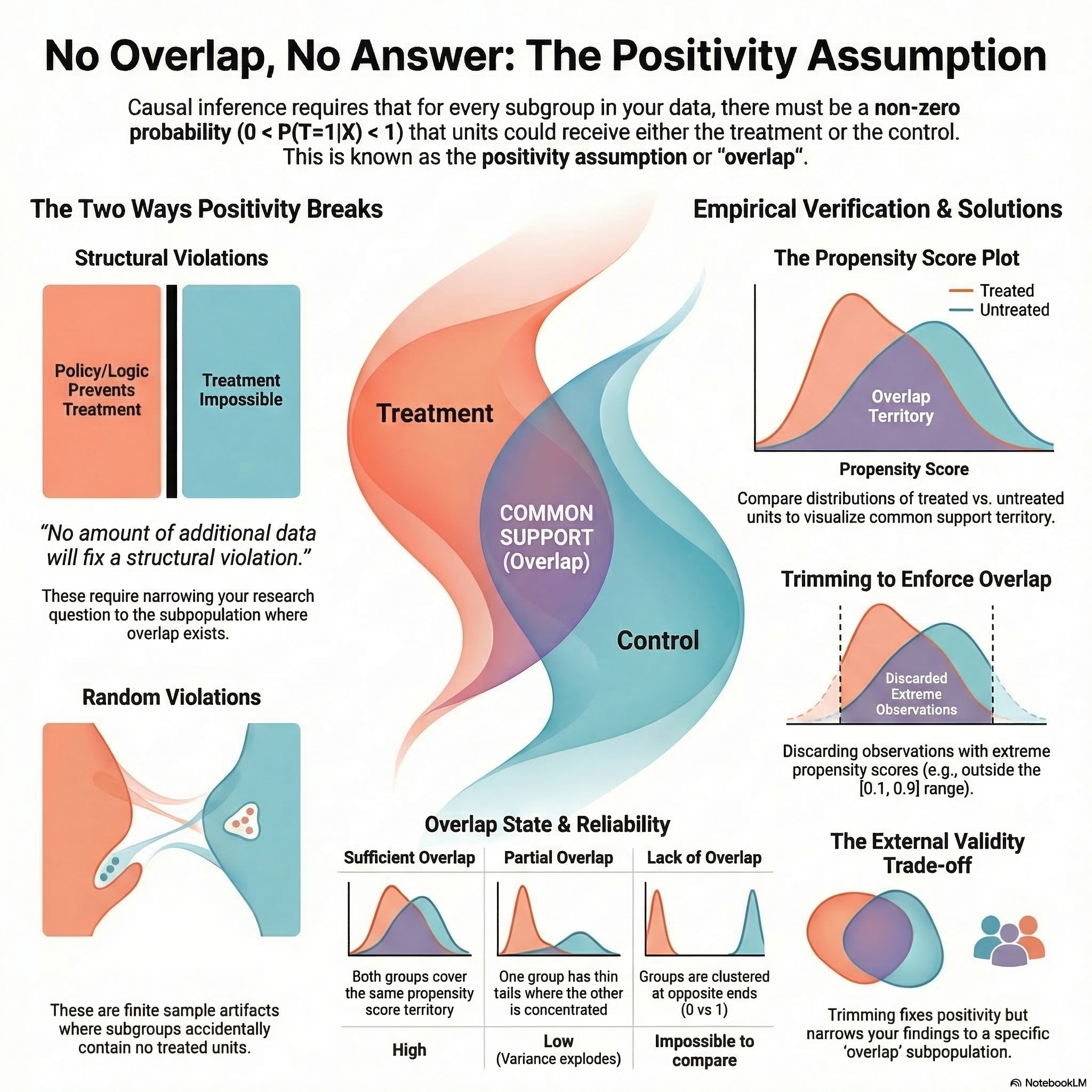
2. Two Ways Positivity Breaks
There are two distinct types of positivity violations (Hernan and Robins 2024):
Structural Violations
These occur when certain units cannot possibly receive a treatment — not because of sample size, but because of logic or policy. In our loyalty programme example, if “Enterprise” status automatically triggers enrollment, the probability of being untreated for that group is zero by design.
The Insight: This is a property of the data-generating process, not the sample. No amount of additional data will fix it. The analysis must be restricted to the subpopulation where positivity holds.
Random Violations
These are artifacts of finite samples. As we condition on more covariates to satisfy exchangeability, we slice the data thinner and thinner. Eventually, we find a cell (e.g., “New users in the UK on iOS”) where, purely by chance, no one joined the programme — even though the true probability in the population is non-zero.
The Insight: These zeros are just bad luck in a small sample. Unlike structural violations, we can often address them using parametric models that smooth over the gaps, borrowing information from adjacent strata. But this comes with a risk: where there is no data, the model is extrapolating — its estimate depends entirely on functional form assumptions, not evidence. A linear model will project a straight line into the gap; a tree-based model will flatline. Neither is learning from data that doesn’t exist.
A practical safeguard: fit multiple model specifications (e.g., logistic regression vs. a generalized additive model with splines) and compare the estimates. If the effect swings wildly between specifications, the extrapolation cannot be trusted.
3. Empirical Verification: Checking for Overlap
How do you know if you have a positivity problem? Unlike exchangeability — which you can never fully verify from data — positivity can sometimes be checked empirically.
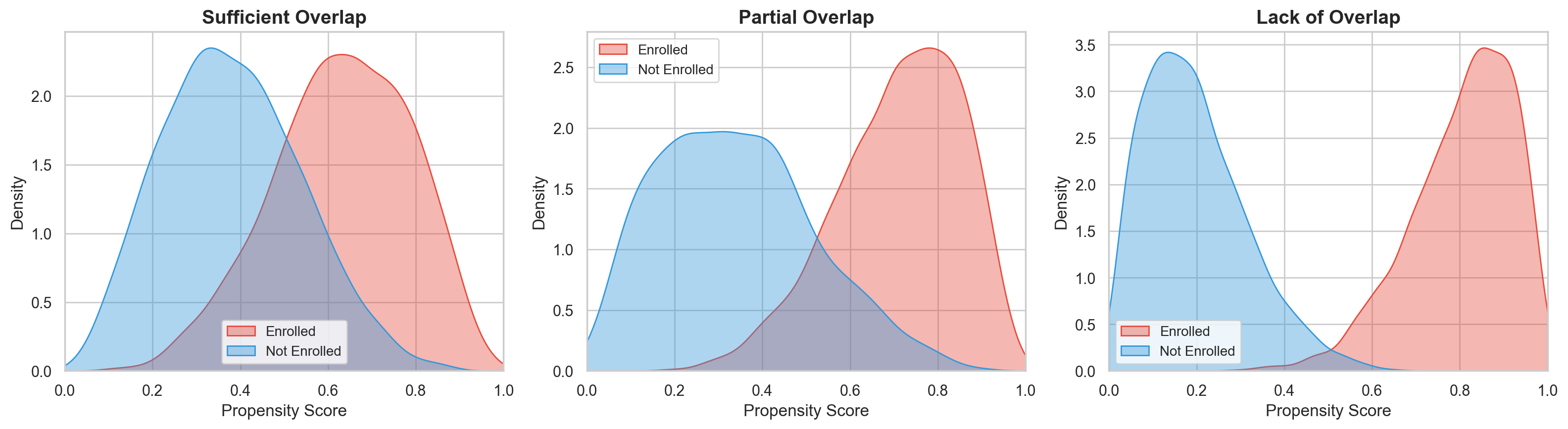
A standard check involves plotting the propensity score distribution separately for treated and untreated units and assessing whether the distributions overlap (Huber 2023). We aren’t looking for identical distributions — only that their ranges cover the same territory. For our loyalty programme, we would estimate each customer’s propensity score — the probability of enrolling given their segment, tenure, and region — then plot the distribution for enrolled vs. unenrolled customers. If the two distributions barely overlap, certain customer profiles have no real comparison group.
- Sufficient Overlap: The ranges of the propensity scores for both groups cover the same territory.
- Partial Overlap: The distributions technically share boundaries, but one group has a thin tail where the other is concentrated. A handful of unenrolled customers at propensity scores above 0.9 can cause variance to explode and hijack the estimate. Check covariate balance specifically in those thin-tail regions to see whether the gap matters for your question.
- Lack of Overlap: One group is clustered near 0 while the other is near 1. The groups are too fundamentally different to be compared.
Ideally, overlap is assessed over the region of the distribution that contains enough observations — not just the extreme points, which may be isolated outliers.
In practice, positivity is enforced by trimming: discarding observations with propensity scores outside a pre-specified interval. A commonly-cited rule of thumb (Crump et al. 2009) is to drop all observations with propensity scores outside \([0.1, 0.9]\). Wider intervals such as \([0.05, 0.95]\) or \([0.01, 0.99]\) are also common.
Who are we actually studying now? What positivity requires depends on the target population. If you care about the effect on treated units only (the ATT), positivity is only needed for the treated subpopulation. If you want the population average treatment effect (ATE), positivity must hold for everyone. Trimming shifts you away from the global ATE — your estimated effect now applies only to the “overlap” subpopulation, not everyone you originally cared about.
Huber (2023) recommends reporting how many observations you dropped so readers understand how much the scope has narrowed.
How aggressively should you trim? It depends on sample size. With more data, extreme propensity scores are more likely to have real counterparts in the other group, so you can afford to trim less. A principled approach — discussed in Huber, Lechner, and Wunsch (2013) and Lechner and Strittmatter (2019) — sets the threshold based on the maximum weight any single observation can carry, rather than a fixed cutoff. This adapts naturally with sample size.
4. Summary
- Positivity requires that every unit has a non-zero probability of receiving each treatment level, for every covariate value present in the population: \(0 < P(T=1 \mid X=x) < 1\).
- Structural violations are business-logic issues that require narrowing your target population.
- Random violations — artifacts of finite samples — are addressed by smoothing with parametric models.
- Positivity can be empirically checked via propensity score overlap plots. Trimming enforces positivity at the cost of external validity.
Keep Going
Up next: The SUTVA Assumption
Exchangeability tells us the groups are comparable. Positivity tells us the comparison is possible. But what if the treatment itself isn’t well-defined — or one unit’s treatment spills over onto another? That’s the challenge of SUTVA.
- EP5: Comparing Apples to Apples — The Exchangeability Assumption — Positivity and exchangeability are complementary. Exchangeability requires comparability; positivity requires that comparisons are possible for every stratum.
- EP4: The Data You’ll Never See — Understanding Potential Outcomes — Positivity is defined in terms of the assignment mechanism and potential outcomes. EP4 introduces the formal language this post relies on.