EP5: Comparing Apples to Apples: The Exchangeability Assumption
Many causal analyses fail not because of bad models, but because of bad comparisons.
Imagine your dashboard flags a troubling trend: users who contacted customer support had a 40% higher churn rate than those who didn’t. The immediate takeaway seems obvious—the support experience is making things worse.
But as experienced practitioners, we know better. Customers usually contact support because something already went wrong—a delayed order, a billing error, or a product defect. The higher churn likely reflects those underlying problems, not the support interaction itself.
The issue isn’t your choice of estimator; it’s that the two groups were never comparable to begin with. This challenge lies at the heart of one of the most critical assumptions in causal inference: Exchangeability.
Listen to This Episode
Want to dive deeper into exchangeability? This podcast episode provides more in-depth information and intuition about the topic. Tune in and follow the podcast to get notified when the next episode is out!
1. The Core Intuition: Apples to Apples
In data science, we often talk about “comparing apples to apples.” In causal inference, Exchangeability is the formal mathematical version of that phrase.
Recall our three primitives from EP4. In our support context:
- Units (\(i\)): Individual customers.
- Treatment (\(T\)): Contacting customer support (\(T=1\)) vs. no contact (\(T=0\)).
- Potential Outcomes (\(Y(1), Y(0)\)): The days to churn if the customer contacts support, and if they do not.
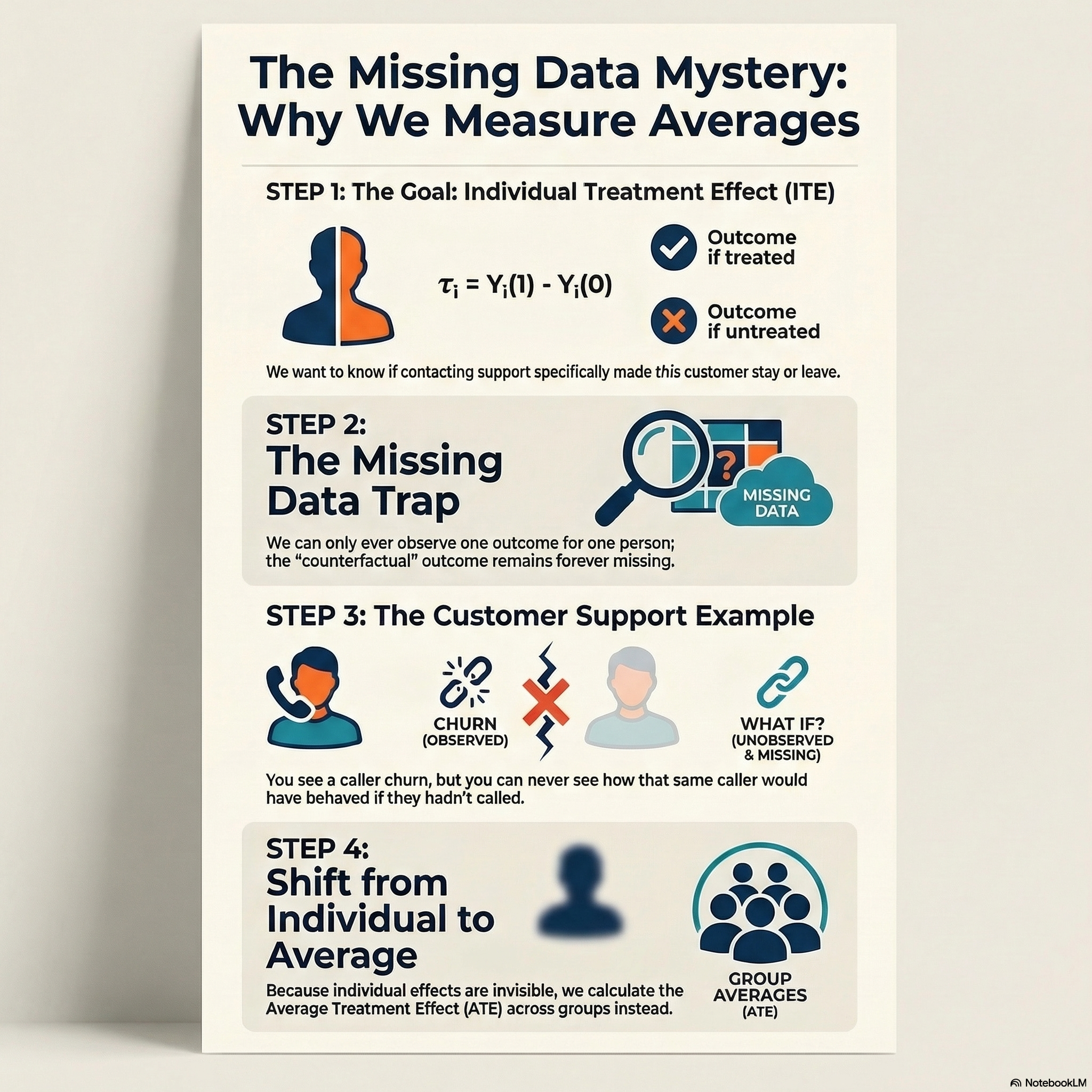
What we really want to know is the individual treatment effect (ITE) — did contacting support make this customer churn sooner or later?
\[\tau_i = Y_i(1) - Y_i(0)\]
To answer that, we would need to observe both potential outcomes for the same customer — but we can only ever observe one. This is the fundamental problem of causal inference (Holland 1986) — at its core, a missing data problem.
Since individual effects are unobservable, we shift our target to the average treatment effect (ATE) across all customers: \[\tau = E[Y_i(1) - Y_i(0)]\]
But here is the catch. To estimate the ATE from observed data, we need the treated and control groups to be truly comparable — so that the control group’s outcomes reflect what the treated group would have experienced without treatment, and vice versa. That is exactly what exchangeability provides.
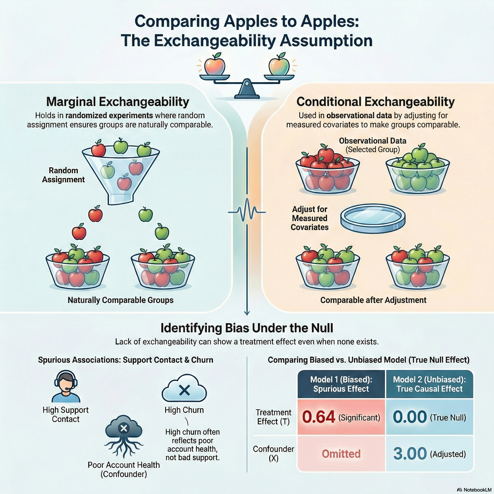
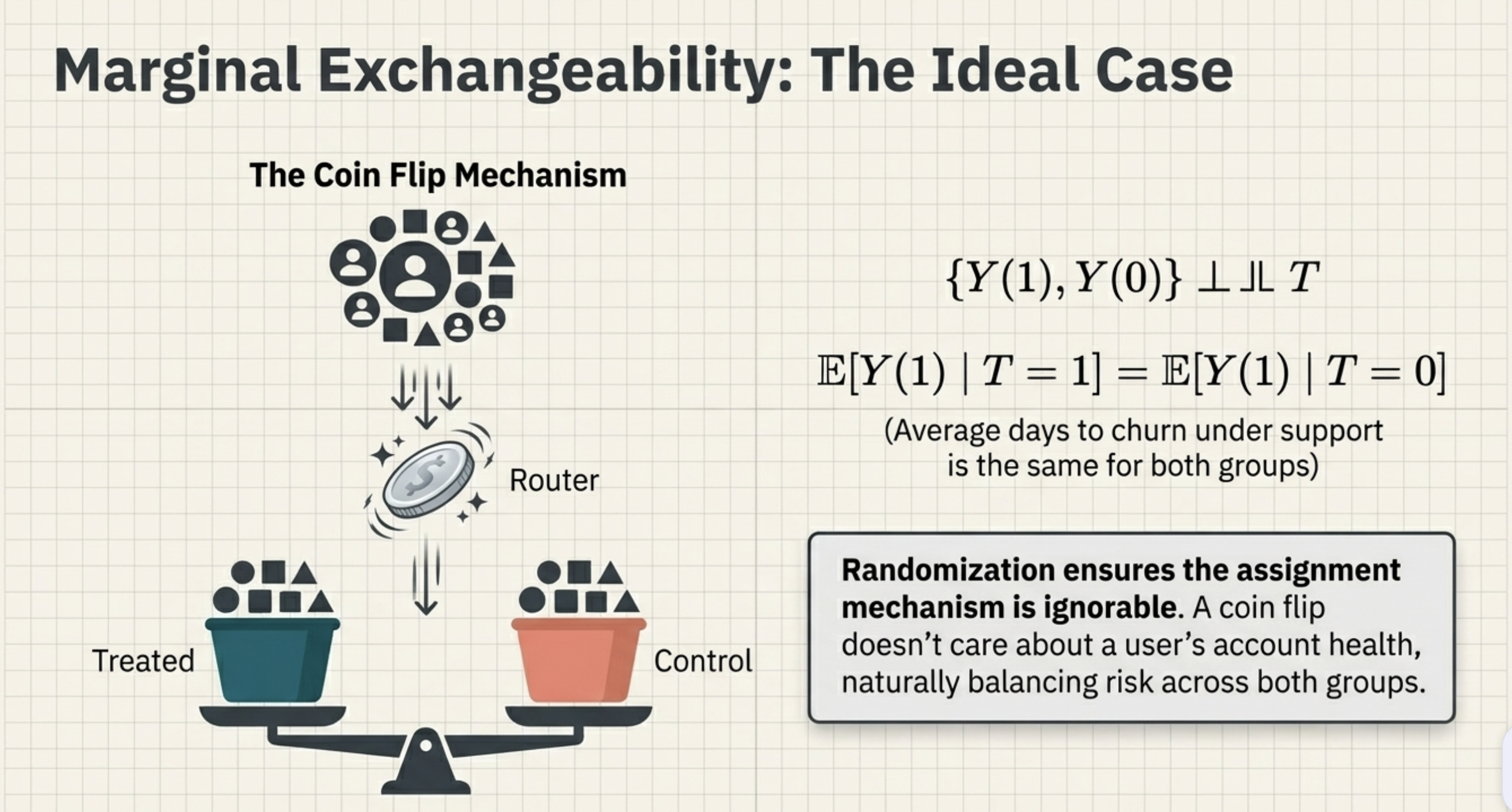
2. Marginal Exchangeability: The Ideal Case
Suppose you could randomly assign customers to contact support or not—perhaps by flipping a coin for every user. Because a coin flip doesn’t care about a user’s billing history or account bugs, it would naturally balance these “risks” across both groups.
The way treatment is assigned to units is called the assignment mechanism (Imbens and Rubin 2010). Randomization ensures the assignment mechanism is ‘unconfounded’ or ‘ignorable’ — the only systematic difference between the groups is the treatment itself. In mathematical notation, we express this using the independence symbol (\(\perp\kern-5pt\perp\)): \[{\{Y(1), Y(0)\} \perp\kern-5pt\perp T}\]
This is Marginal Exchangeability. It means if you swapped the groups, the average outcomes wouldn’t change. You are comparing Apples to Apples: \[E[Y(1)\mid T=1] = E[Y(1)\mid T=0]\] In words: the average days to churn under support contact is the same for customers who actually contacted support (\(T=1\)) and those who did not (\(T=0\)). \[E[Y(0)\mid T=0] = E[Y(0)\mid T=1]\] And likewise: the average days to churn without support contact is the same for both groups.
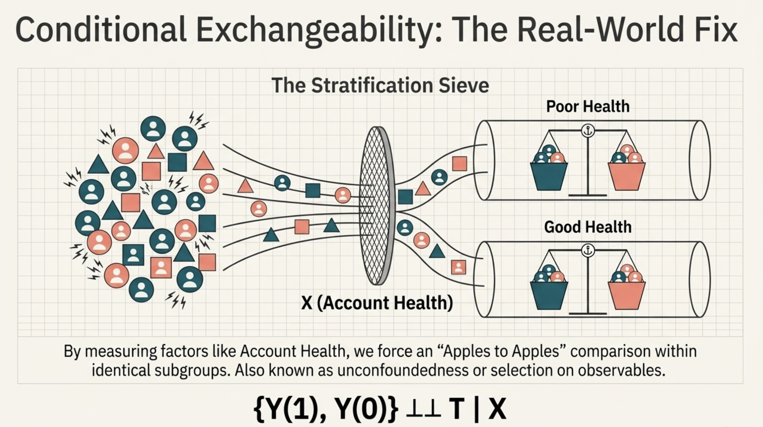
3. Conditional Exchangeability: The Real World
In practice, we cannot randomize customer support. We cannot logically “flip a coin” to decide which users get help and which are ignored when their product breaks.
Instead, users “select” into treatment based on their needs. A user with a broken product is much more likely to reach out. Comparing these users to “healthy” users who didn’t need support is comparing Apples to Oranges. The groups are no longer exchangeable.
The following causal graph captures this situation. Account health (\(X\)) affects both whether a customer contacts support (\(T\)) and whether they churn (\(Y\)). It is a common cause of treatment and outcome — a confounder.
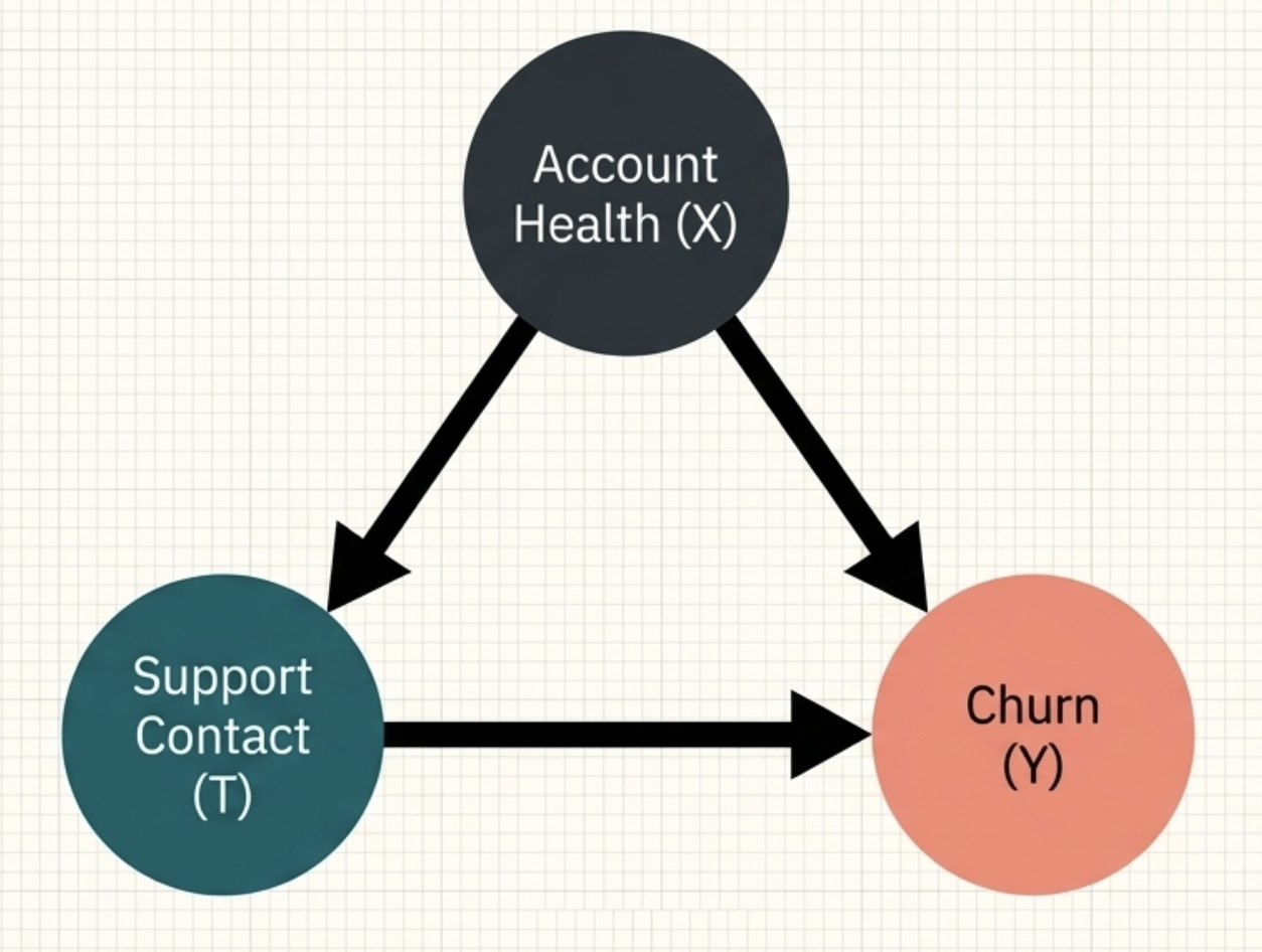
However, if we can measure the factors that influence both contact and churn—like Account Health (\(X\))—we can restore the balance. Among users with identical “Poor Health” scores, some will contact support and some won’t. Within this specific subgroup, the comparison becomes fair again.
This is Conditional Exchangeability. Using the same independence notation as before: \[{\{Y(1), Y(0)\} \perp\kern-5pt\perp T \mid X}\]
Once we adjust for \(X\), we have forced an “Apples to Apples” comparison. This assumption is also known as unconfoundedness (popular among epidemiologists), selection on observables (popular among social scientists), or simply conditional independence (Ding 2023).
4. Empirical Proof: Bias Under the Null
Confounding is dangerous because it creates a “finding” even when the treatment has zero effect. This is called bias under the null (Hernan and Robins 2024).
Let’s demonstrate this empirically. We generate simulated data where support contact genuinely has no effect on when users churn (a null causal effect), and account health is the only confounder.
- Model 1 (Naive): We ignore account health. The model shows a statistically significant correlation between support and churn.
- Model 2 (Adjusted): We condition on account health. The spurious effect disappears, revealing the truth.
In the table below, Support Contact corresponds to treatment \(T\), Account Health corresponds to the confounder \(X\), and the Intercept represents the baseline expected days to churn when both are zero.
| Variable | Model 1 (Naive) | Model 2 (Adjusted) |
|---|---|---|
| Intercept | 2.12*** | 1.00*** |
| Support Contact (T) | 0.64* (Spurious)** | 0.00 (Truth) |
| Account Health (X) | - | 3.00*** |
Note: The DGP implements the causal structure in the graph above with a null causal effect between \(T\) and \(Y\). Support contact is a binary treatment variable, days to churn is the continuous outcome, and account health is a binary confounding variable drawn from a binomial distribution.
Without exchangeability, we cannot identify the true (null) causal effect. The model is simply reporting selection bias — the pre-existing differences in your user base.
In observational data, the treated group is rarely a random draw — it is a selected group. Conditioning on \(X\) helps restore exchangeability, but only to the extent that your measured covariates capture the systematic reasons the treated and untreated groups differ. If an important confounder is unmeasured, the estimate will be biased — and we cannot fully trust the results.
The practical question is not simply whether to condition, but what to condition on — a question that causal graphs, covered in a later episode, will answer precisely. And when you suspect unmeasured confounders may remain, sensitivity analysis can help assess how robust your conclusions are — we will cover this in a later episode as well.
5. Identification Strategies in Context
Exchangeability is the bedrock of the conditioning family — methods like regression adjustment, (propensity score) matching, and inverse probability weighting. But it is not a universal requirement for causal identification. It is the price of using a conditioning strategy specifically.
Other strategies take a different path under different assumptions:
| Strategy | Logic | Core Assumption |
|---|---|---|
| Conditioning | Adjust for \(X\) to make groups comparable. | Exchangeability given \(X\). |
| Diff-in-Diff | Compare the change over time. | Parallel Trends. |
| Instr. Variables | Use a “random glitch” to trigger treatment. | Exclusion Restriction. |
| Reg. Discontinuity | Compare users just above/below a threshold. | Continuity. |
The right choice depends on your data and which assumptions are most defensible in your context. We will cover each of these strategies in later episodes.
6. Summary
- Exchangeability is the formal requirement for an “Apples to Apples” comparison.
- Randomization gives us this for free, but is often impossible in real-world product settings.
- Conditioning is how we try to “force” exchangeability in observational data by adjusting for confounders.
- Bias Under the Null is why we can’t trust correlations: your model may show an effect simply because the groups were different to start with.
- Deciding what covariates to condition on is the central challenge of the conditioning strategy. Causal graphs, covered in a later episode, provide the principled tool for making this decision.
Keep Going
Up next (EP6): The Positivity Assumption
Exchangeability tells us the groups are comparable. But what if there are certain types of “at-risk” users who always contact support? If there’s no one in the control group to compare them to, we can’t estimate the effect. That is the challenge of Positivity.
- EP2: The Bridge to Truth — Why Identification Comes Before Estimation — Exchangeability is one of the identifying assumptions introduced in EP2. If you want the full picture of what identification requires, EP2 is the foundation.
- EP4: The Data You’ll Never See — Understanding Potential Outcomes — Exchangeability is defined in terms of potential outcomes. EP4 builds the formal language — potential outcomes, the ATE, and the fundamental problem of causal inference — that this post relies on.