EP4: The Data You’ll Never See: Understanding Potential Outcomes

1. The Data You’ll Never See

You can never see the data you need most to make a decision.

Most data science focuses on predicting the future from what happened in the past. Causal inference asks a harder question: what would have happened if we had acted differently?

The Discount Trap

Your retention team sends a 20% discount to at-risk subscribers. Churn drops. Everyone celebrates.

But then a skeptical stakeholder asks the uncomfortable question: were those customers actually going to churn — or were they going to renew anyway, and you just gave away 20% of their revenue for nothing?

This is the fundamental problem of causal inference. You observe that a customer received the discount and renewed — their outcome under treatment, \(Y(1)\). But the counterfactual — whether that same customer would have renewed without the discount, \(Y(0)\) — is forever hidden. You can never send and not-send the discount to the same customer simultaneously.

Without a formal language for these unobserved parallel worlds, you cannot even precisely define what “the effect of the discount” means, let alone estimate it.

Potential Outcomes: Naming the Invisible

Potential outcomes provide the formal language to make this precise: they give a name and a mathematical slot to both the outcome you observed and the one you didn’t — turning the unobserved counterfactual into a concrete object you can reason about.

In this episode, we cover: potential outcomes, individual treatment effect (ITE), the fundamental problem of causal inference, and the three basic primitives — units, treatments, and potential outcomes.

The potential outcomes framework at a glance.

Listen to This Episode

Want to dive deeper into potential outcomes? This podcast episode provides more in-depth information and intuition about the topic. Tune in and follow the podcast to get notified when the next episode is out!

2. Potential Outcomes: A Baking Example

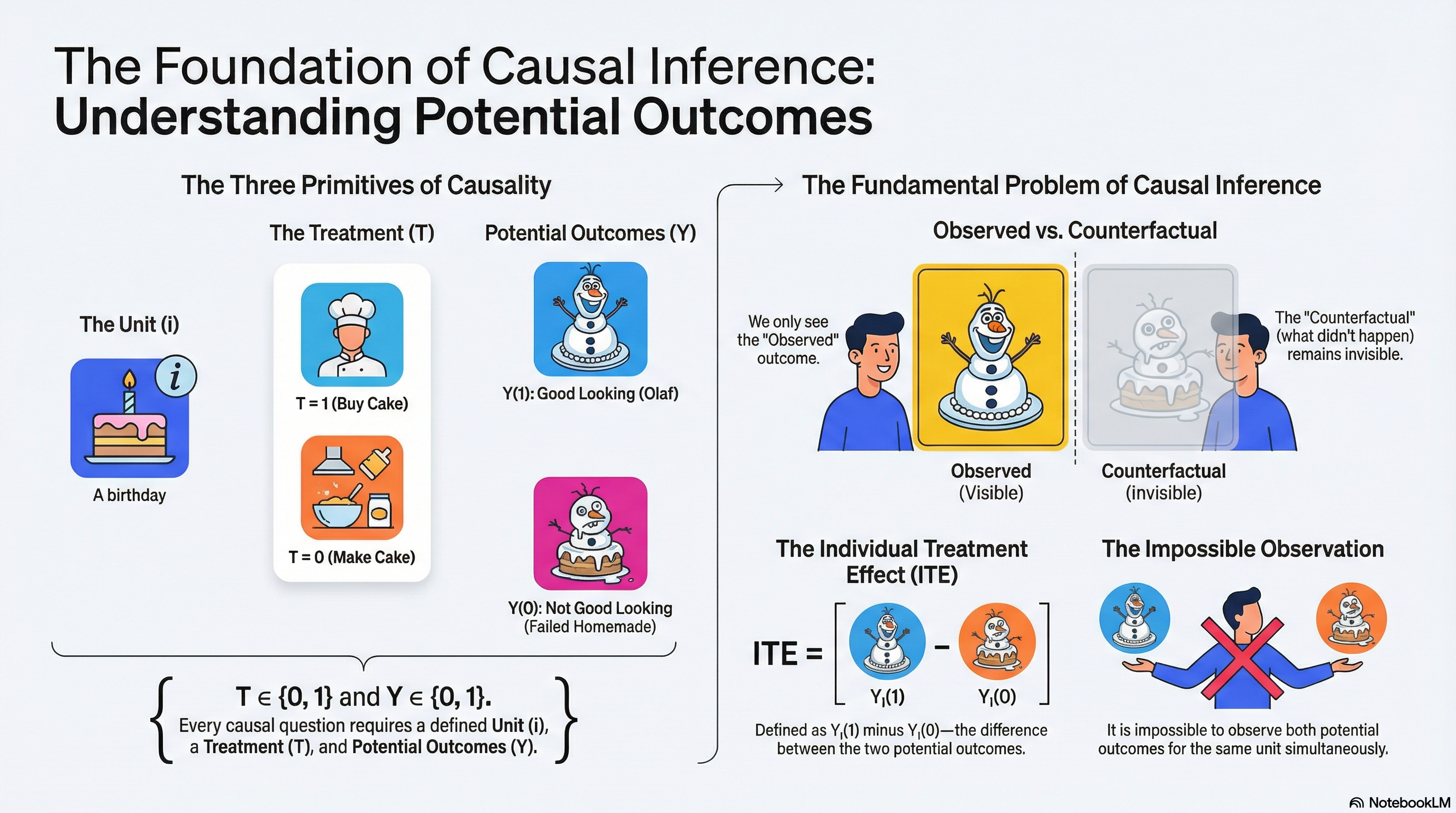
I’m interested in the causal question: Does buying a birthday cake from a cake shop improve the cake’s look vs a homemade cake? ¹

In this example, the treatment is buying a cake from a cake shop or making a cake at home (\(T∈\{0, 1\}\)). The outcome is we thought the cake looked good or bad (\(Y∈\{0,1\}\)). For this birthday occasion, since we actually bought the cake from the cake shop, my cake looks like Figure 1. We can write the outcome for \(T = 1\) as \(Y(1)\). We think the cake looks good, so \(Y(1) = 1\). This is the observed outcome.

Figure 1. \(Y(1) =1\), buying a birthday cake from cake shop \(T=1\) leads to a good looking cake \(Y=1\)

To know if the cake was looking good because it was made in a cake shop rather than made at home (in which case there is a causal effect), I would have needed to know the look it would have had, had my family made it at home \(Y(0)\) (maybe Figure 2, however, this is unobserved in this birthday occasion).

Figure 2. \(Y(0) = 0\), making a birthday cake at home \(T=0\) leads to a not so good looking cake \(Y=0\)

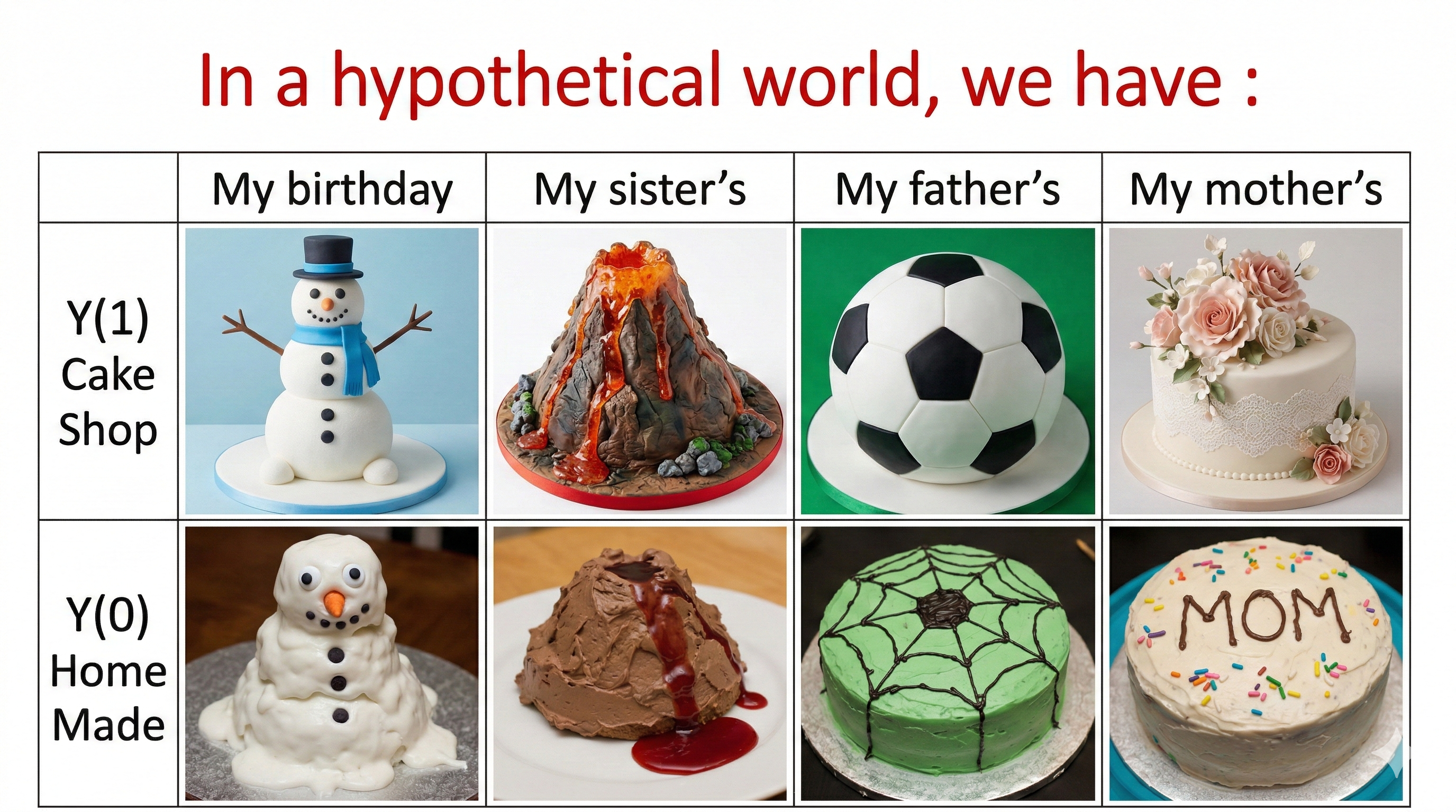
Let’s say that our units of analysis are the birthdays of n different people. We know that to answer the causal question of interest, we would ideally observe both the birthday cake bought from cake shop \(Y(1)\), and birthday cake made at home and \(Y(0)\), for all different people such as shown in Figure 3.

Figure 3. Hypothetical world cake shop example

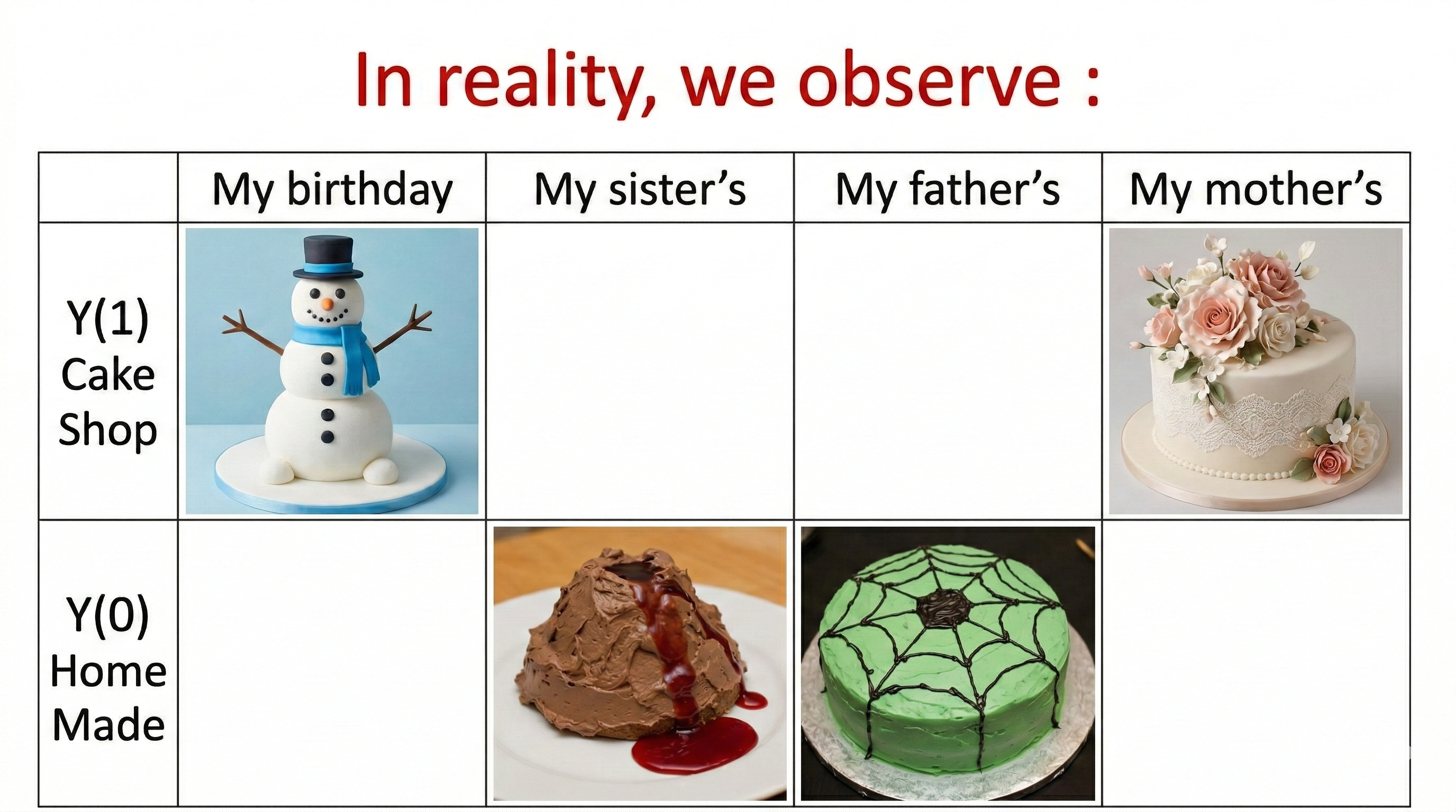
However, in reality, we would only observe one of the potential outcomes for different people as in Figure 4, either \(Y(1)\) or \(Y(0)\).

Figure 4. Real world cake shop example

3. Potential Outcome Definitions and Three Primitives

More generally, the potential outcome \(Y(t)\) denotes what our outcome would be, if we were to take treatment \(T = t\). A potential outcome \(Y(t)\) is distinct from the observed outcome because not all potential outcomes are observed. Rather, all potential outcomes can potentially be observed — the one that is actually observed depends on the value that the treatment takes on.

For defining causal effects, there are three basic primitives – concepts that are fundamental and on which we must build: units, treatments and potential outcomes(Imbens and Rubin 2010).

• A unit is a physical object, for example, a customer, a trip that customer takes at a particular point in time. We have a set of units indexed by \(i\).

• A treatment is an action that can be applied or withheld from a unit. We usually focus on the case of two treatments². Let \(T_{i}\) be the value of a treatment assigned to individual \(i\).³

• Associated with each unit are two potential outcomes: the value of an outcome variable \(Y\) if the active treatment \(T=1\) is taken on \(Y_{i}(1)\), and the value of \(Y\) if instead the control treatment \(T=0\) is taken on \(Y_{i}(0)\).

These concepts are not just theoretical concepts. In our empirical causal analysis, it is also crucial to address the 3 concepts explicitly.

4. Individual Treatment Effect and the Fundamental Problem of Causal Inference

Potential outcomes enable us to translate causal questions into the estimation of a causal estimand. For each individual \(i\), the outcome of interest \(Y\) has two versions: \(Y_{i}(1)\) and \(Y_{i}(0)\)⁴. We can define the Individual Treatment Effect (ITE) \(\tau_{i}\) as the difference⁵.

\[\tau_{i}= Y_{i}(1) -Y_{i}(0)\]

The objective is to learn about the causal effect of the active treatment relative to the control on Y, where, by definition, the causal effect is a comparison of the two potential outcomes⁶. However, it is impossible to observe the value of \(Y_{i}(1)\) and \(Y_{i}(0)\) for the same unit. Therefore, it is impossible to observe the ITE. Hence we run into the fundamental problem of causal inference(Holland 1986), namely, we cannot observe the counterfactual.

To get around the fundamental problem of causal inference, instead we can focus on the average treatment effect across the different units, which is a causal estimand (for an introduction to causal estimands, see EP1): \[\tau= E[Y_{i}(1) -Y_{i}(0)]\]

To use the causal estimand average treatment effect to answer the causal question, we need to make stringent assumptions and evaluate explicitly whether these assumptions are realistic in our practical work. We will cover these assumptions in the next episodes.

5. Practical Example: Customer Churn and Discount Offers

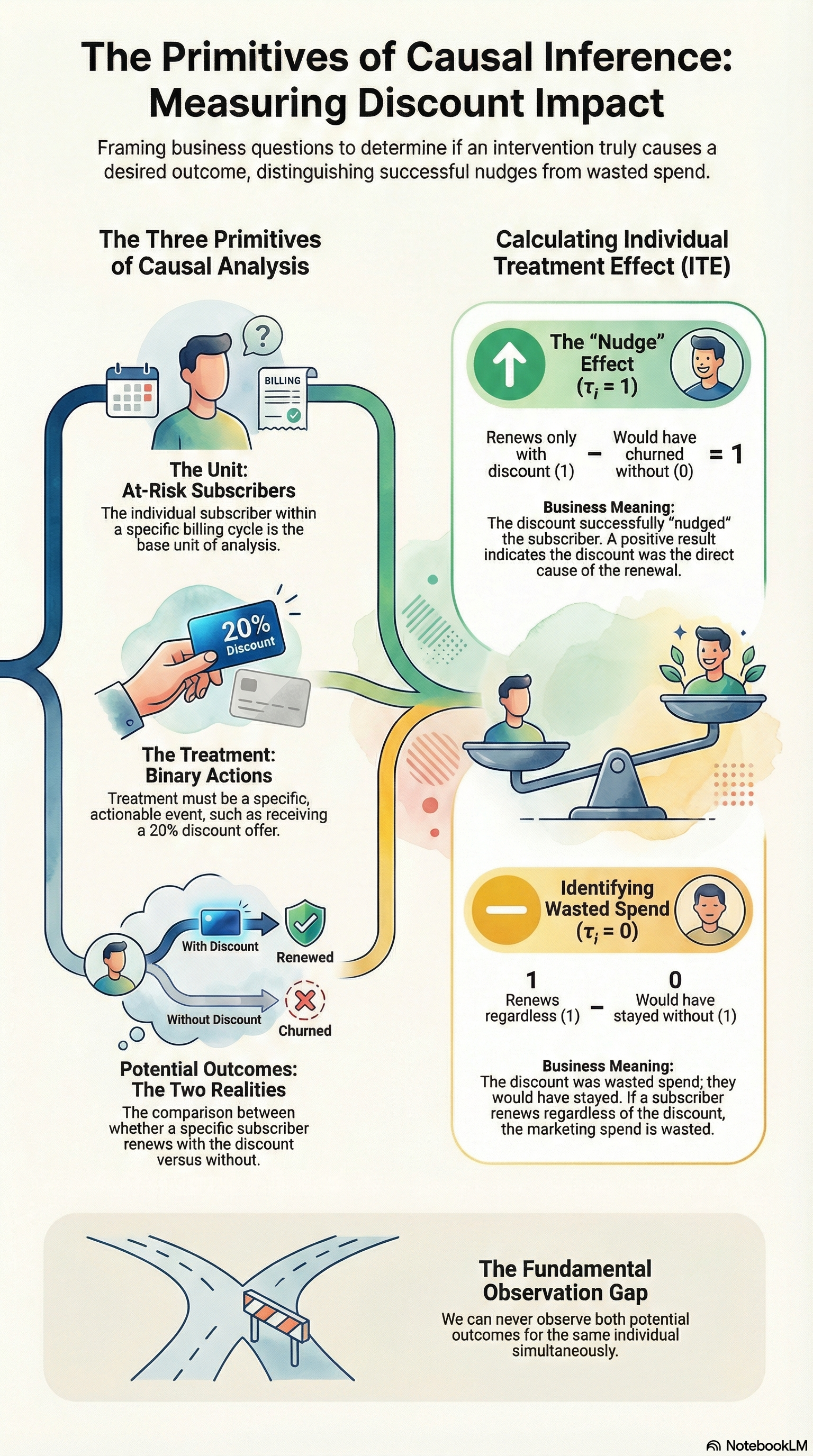
Let’s return to the discount example from the opening and apply the three primitives formally. The causal question: does offering a 20% discount to at-risk subscribers reduce churn?⁷

• Units: the unit of analysis is a subscriber flagged as at-risk within a given billing period. Using the subscriber as the unit makes sense because the treatment — receiving a discount — is applied once per billing cycle per subscriber.

• Treatment: the treatment is receiving a 20% discount offer (\(T=1\)) vs. receiving no discount (\(T=0\)). The treatment must be a clearly defined action: “received a discount offer” is specific and actionable; “being a loyal customer” is not.

• Potential Outcomes: \(Y_i(1)\) is whether subscriber \(i\) renews their subscription if offered the discount; \(Y_i(0)\) is whether subscriber \(i\) renews if not offered the discount.

The ITE for subscriber \(i\) is:

\[\tau_i = Y_i(1) - Y_i(0)\]

This is the answer to the question we actually care about: did the discount cause this specific subscriber to stay? A subscriber with \(\tau_i = 1\) genuinely needed the nudge. A subscriber with \(\tau_i = 0\) would have renewed regardless — meaning the discount was wasted spend. We can never observe both values for the same subscriber, but naming them precisely is what makes the problem tractable.

Figure 5. Potential outcomes for whether offering a 20% discount to at-risk subscribers reduces churn.

DS Translation: From Primitives to Decisions

Grounding the three primitives explicitly is not a formality — it is the first concrete check on whether your analysis can deliver a causal answer.

• Unit choice determines what counts as one observation. Using subscribers flagged as at-risk per billing period avoids conflating different risk profiles or time windows for the same customer.
• Treatment definition must describe a clearly actionable intervention. “Received a discount offer” is specific; “being a high-value customer” is not — you can’t randomise a characteristic.
• Potential outcomes force you to ask: what would this subscriber have done under the alternative? That question surfaces confounding risk before you touch a model — and in this case immediately flags that high-intent subscribers are more likely to both receive and not need the discount.

In practice, teams that skip this step often discover halfway through an analysis that the treatment is ill-defined or the unit of analysis conflates different populations. Defining primitives first is cheap; discovering the problem last is not.

6. Summary

In this episode, we built the formal language for causal questions. Starting from the discount trap — where observed outcomes alone can’t tell you whether a treatment worked — we introduced potential outcomes as the tool for naming what we observe and what we don’t. We then grounded the framework in three primitives every causal analysis must define, and showed why individual causal effects are unobservable in principle, pushing us toward population-level estimands.

1. Potential outcomes \(Y_i(1)\) and \(Y_i(0)\) give us a formal language for what we want to know but can never fully observe for the same unit at the same time.
2. The three primitives — units, treatments, and potential outcomes — must be defined explicitly before any causal analysis.
3. The Individual Treatment Effect \(\tau_i = Y_i(1) - Y_i(0)\) cannot be observed for any single unit — this is the fundamental problem of causal inference.
4. Instead, we target the Average Treatment Effect \(\tau = E[Y_i(1) - Y_i(0)]\), which requires stringent assumptions we will unpack in the next episode.

Keep Going

Up next (EP5): Exchangeability Assumption

We now have a precise definition of the ATE — but defining it and estimating it are two different things. The key assumption that bridges the gap is exchangeability (also known as no unmeasured confounding or ignorability): the condition under which the observed difference between treated and untreated groups actually equals the causal effect we care about.

Without it, even a perfect dataset gives the wrong answer. With it, the ATE becomes estimable from observed data — and conditioning strategies like regression adjustment, matching, and inverse probability weighting become valid. Exchangeability is the signature assumption of the conditioning family, and understanding it precisely is what separates rigorous causal analysis from sophisticated correlation.

Exchangeability is one of three assumptions required for identification by conditioning. The other two are covered in subsequent episodes:

• Stable Unit Treatment Value Assumption (aka SUTVA) — ensures that potential outcomes are well-defined: there are no spillovers between units (non-interference) and the treatment has a single, unambiguous version (consistency).
• Positivity — ensures that every unit has a positive probability of receiving either treatment, so the ATE is actually estimable across the full population.

Recommended background (optional)

This episode sits at the intersection of three foundations built earlier in the series. EP1 gave us the vocabulary for what we are trying to estimate; EP2 showed why that estimate cannot come from data alone without assumptions; EP3 explained why causal questions require a different mode of reasoning than prediction. Potential outcomes are the formal language that makes all three of those ideas precise.

• EP1: The Core Trio — Estimand, Estimator, Estimate The ATE introduced here is a causal estimand. EP1 builds the vocabulary — estimand, estimator, estimate — that gives the ATE its precise meaning, and explains why defining the quantity of interest must come before any computation.

• EP2: The Bridge to Truth — Why Identification Comes Before Estimation EP4 defines what we want — the ATE expressed in potential outcomes. EP2 addresses the next question: under what conditions can that causal estimand actually be recovered from data? It introduces identification as the critical bridge between counterfactual quantities and observable evidence.

• EP3: The Ladder of Causation EP4 provides the formal language for the intervention questions that EP3 named. The Causal Hierarchy explains why we need potential outcomes at all — prediction tools answer Level 1 questions, but causal decisions live at Level 2, which requires the counterfactual reasoning that potential outcomes make precise.

References

Dumas, Elise. 2023. “Introduction to Causal Inference - Tools for Causality, Thematic Quarter on Causality.” Introduction to Causal Inference. https://quarter-on-causality.github.io/tools/intro_causal_inference_elise_dumas.pdf.

Fisher, Sir Ronald Aylmer. 1935. The Design of Experiments. Oliver; Boyd.

Holland, Paul W. 1986. “Statistics and Causal Inference.” Journal of the American Statistical Association 81 (396): 945–60. https://doi.org/10.2307/2289064.

Imbens, Guido W., and Donald B Rubin. 2010. “Rubin Causal Model.” In Microeconometrics, edited by Steven N. Durlauf and Lawrence E. Blume, 229–41. London: Palgrave Macmillan UK. https://doi.org/10.1057/9780230280816.

Neyman, J. 1923. “On the Application of Probability Theory to Agricultural Experiments. Essay on Principles (with Discussion). Section 9 (Translated). Reprinted Ed.” Statistical Science 5: 465–72.

Pearl, Judea. 2000. Causality: Models, Reasoning, and Inference. Cambridge University Press.

Rubin, Donald B. 1974. “Estimating Causal Effects of Treatments in Randomized and Nonrandomized Studies.” Journal of Educational Psychology 66 (5): 688–701. https://doi.org/10.1037/h0037350.

Footnotes

1. The example is just for illustration purposes. The birthday cake is inspired by Dumas (2023).

2. Although the extension to more than two treatments is simple in principle, it is not necessarily so with real data.

3. The emphasis on action is deliberate. Holland’s (1986) principle — “no causation without manipulation” — requires that a treatment correspond to a coherent intervention that can, in principle, be applied or withheld. Fixed attributes such as height or a customer’s inherent loyalty are not directly manipulable: the potential outcome \(Y_i(t)\) is ill-defined when there is no clear mechanism that sets \(T=t\). We will formalise this under the well-defined treatment assumption (consistency/SUTVA) in EP5.

4. It seems intuitive but has some hidden assumptions — specifically consistency (SUTVA), exchangeability, and positivity — which we will cover in the following post.

5. We can also consider other quantities than the difference, such as the ratio, or the percentage increase due to treatment. In any case, it is some contrast measure between two potential outcomes.

6. Potential outcome is one common way to express counterfactual statements as probability quantities. It originated from Neyman (1923) and Fisher (1935) work on understanding experiments. Later on, Donald Rubin formalized it in a series of famous papers (1st one in 1974)(Rubin 1974). Potential Outcomes has evolved into an entire framework for causal inquiry. An alternative way to express counterfactual in probability is Judea Pearl’s do operator (Pearl 2000)

7. This use case is for illustrative purposes and does not explicitly consider all assumptions.

Copyright

© 2026 Lin Jia. All rights reserved. This content is created independently on personal time and is based exclusively on public domain academic knowledge. No proprietary, confidential, or employer-owned materials, data, or intellectual property are included. The views and opinions expressed in this work are strictly my own and do not reflect those of any current or former employer. All methodology discussed is sourced from publicly available scientific literature.