Ask the room: hands up if you have shipped a feature people had to opt in to. Keep referring back to their feature.

This isn't one product's problem. It's structural, and it hits both sides of a marketplace.

Demand side: travellers choose whether to log in, claim a discount, join a loyalty programme. Supply side: partners choose whether to enable smart pricing, activate instant booking, adopt an optimisation tool.

The contrast that matters: change a search ranking and it applies to 100% of traffic immediately. An opt-in feature applies only to whoever chooses it — and we cannot force that choice.

Here is the whole talk in one slide.

Story A: the feature genuinely doesn't work — nobody benefits, kill it. Story B: it works brilliantly, but almost nobody adopted it — so fix the funnel, not the product.

A flat A/B test looks identical in both cases. And the two answers point to opposite decisions — kill it, or invest in adoption. That ambiguity is what we're going to resolve.

If someone is thinking "or your metric was wrong, or the test was underpowered, or it only worked for one segment" — yes, and we rule those out in the next few slides. The point here is that even with a clean, well-powered test, these two stories still look the same.

Three problems, and they compound.

In the Medium post we call this the opt-in trilemma — the term is optional out loud

1 — Voluntary adoption. Users actively choose. A standard A/B test cannot separate the product's effect from the motivation that drove someone to adopt in the first place.

2 — Heterogeneity. Our partners run from single-apartment hosts to global chains; travellers from once-a-year holidaymakers to agencies booking thousands of nights. Huge variance on both sides.

3 — Finite sample. Opt-in features target sub-segments. The eligible population is finite, so "run it longer" is not available as a fix for low power.

"Success" here is really two questions, and they are not the same question.

Question 1 — overall impact. Your success metric across the whole eligible group — adopters and non-adopters together. That is what leadership is asking about when they ask whether shipping it was worth it.

Question 2 — impact on adopters. The same success metric, but only for the people who actually adopt it — whatever adopting means for your feature. That is what tells you whether the thing you built works, and whether to keep building it.

Keep both in mind. The next two slides show that the first one is straightforward — a standard A/B test answers it, just very diluted. Then we spend most of the talk on the second, because that is where it gets hard.

No jargon yet — both numbers get their proper names later

A hypothetical supply-side scenario, inspired by a real class of problem.

What the tool does. Every partner manages inventory settings by hand — which dates are open, how short a stay they accept, what they charge. The tool takes that over: it tunes those settings automatically, every day, per property, to keep the listing competitive. The payoff for the partner is fewer empty nights.

The outcome we measure is bookings per partner — the core volume metric for supply-side products.

Two numbers to hold on to. Half of the eligible partners are randomly offered the tool. Of those, only about one in ten actually adopts it — switches it on. That 10% is what drives everything that follows.

Both of the questions from the last slide are now concrete: what did offering this tool deliver across everyone, and what did it deliver for the partners who adopted it.

Say out loud: all numbers are illustrative  ·  ⏱ ~05:00 when leaving this slide

Start with the good news: for question 1 — the overall impact — a standard A/B test is exactly the right tool.

The two groups. Half were offered the tool, half were blocked. A coin decided which. So the two groups are alike in every way, observed and unobserved — and the gap between their averages is an unbiased estimate of what offering the tool delivered. No modelling, no assumptions. This is the measurement A/B testing does correctly.

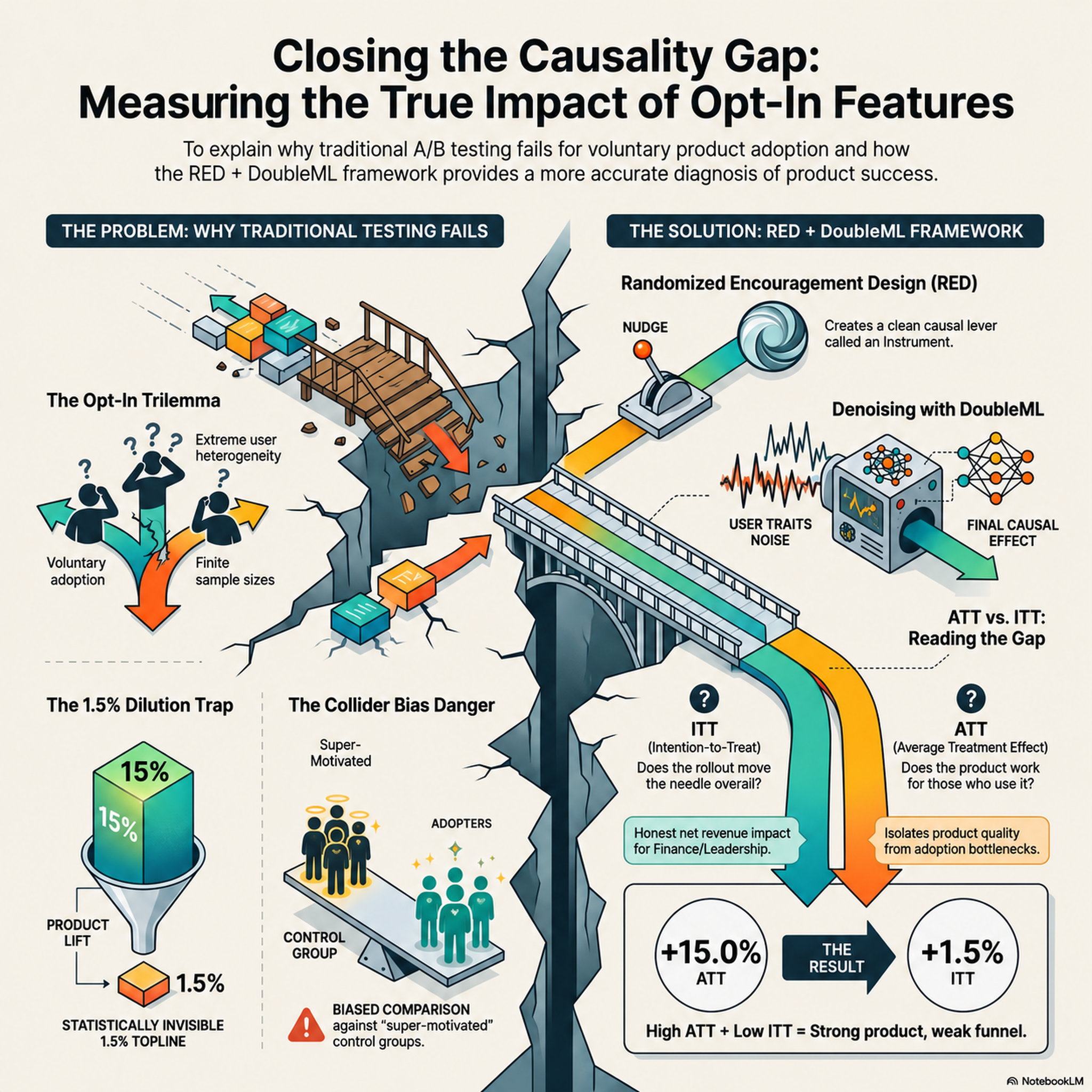
Now the bad news. That gap averages over everyone who was offered it, adopters and non-adopters together. One in ten adopted and gained 15%; the other nine contribute zero. So 0.10 × 0.15 gives a 1.5% gap.

Against real-world variance, 1.5% is statistically indistinguishable from zero. The measurement is correct and the test still comes back flat — the feature looks like it did nothing.

So question 1 is handled. What we do not have is question 2: the impact on the people who adopted. That is the rest of the talk.

Both numbers get their proper names later — no ITT / ATT yet

For the adopters, what we want is a counterfactual: what would this same partner have done without the tool? We cannot observe that. So the natural move is to find a stand-in.

For every adopter, find a non-adopter who looks the same on everything we can see — size, city, past bookings. Treat the twin as the adopter's what-if. Compare the two, and it feels as if we had randomised who got the tool. The logic feels airtight.

Three common implementations: regression adjustment with adoption and covariates as controls; propensity score matching or inverse probability weighting; or naive DoubleML using ML to partial out covariates (PLR / IRM architectures).

They are not really three methods. Every one of them estimates the same contrast: outcomes of adopters against outcomes of matched non-adopters. They differ only in how they weight that comparison — so whatever bias is in the contrast, all of them inherit it.

Name the assumption out loud: the twin is only a valid what-if if the columns we matched on are everything that separates an adopter from a non-adopter. Hold that thought — the next slide tests it, and the one after that shows what breaks.

Chernozhukov et al. 2018 — cite if asked

Lin takes over here

Same ten partners. Let me make the motivation gap concrete.

Left — no tool yet. Nine partners book about 100. The red flame is the motivated one: responds to demand faster, keeps the calendar tidy. That partner already books 120 — nothing to do with any tool. And "motivated" is not a column in our data.

Right — offer the tool. Who adopts? The motivated one. The tool genuinely adds 15, so that partner goes to 135. Compare adopters to non-adopters and you measure 135 against 100: a gap of 35.

35 = 15 of tool + 20 of motivation — and the 20 was there before the tool existed. Regression, matching, IPW, naive DoubleML all measure the 35. None can subtract the 20, because the thing that would let them is not recorded.

If the hidden variable is the problem, stop adjusting for it. Go back to the one clean thing: the coin. And we already flipped it. Remember the A/B test: half the partners got the offer, half did not. That is a randomised encouragement design — and it is a textbook instrumental variable. The offer is the instrument, adoption is the treatment.

We cannot force adoption. But we can randomise the offer — feature access, a notification, a voucher. Anything that raises the chance of adopting without forcing it. That is an instrumental variable, and it needs three things, one per card.

Why "instrument"? Because it is a tool, not the thing we care about. We do not care about the offer's effect on bookings for its own sake. We use the offer as a lever to create clean, random variation in adoption, then read the effect of adoption off that variation. "Instrument" in the old sense of a measuring device — like a thermometer for temperature. The term dates to 1920s econometrics: Philip Wright used weather as an instrument to trace supply curves in 1928.

Walk the graph: the offer shifts adoption; adoption shifts bookings; and there is no direct route from offer to bookings. So any offer–bookings correlation must flow through adoption. Motivation is still out there, still unobserved — but the offer was a coin flip, so nothing connects them. We did not remove the confounder; we made it irrelevant.

The crucial move: we never compare adopters to non-adopters. We compare the whole offered group with the whole blocked group — the comparison the coin guarantees is fair. Both groups hold the same share of willing partners; only in the offered group did they actually use the tool.

Next slide: divide by the share who adopted, and the per-adopter effect falls out.

⏱ ~12:00 entering this slide

One randomised encouragement design answers both questions we started with, and it takes one division.

ITT — offered group minus blocked group: 1.5%. Whole groups, randomisation intact. That is the net rollout impact, the number Finance needs.

ATT — every booking the offer caused went through the 10% who adopted, so 1.5 over 0.10 is 15% per adopter. That is the number Product needs. Because the blocked group cannot adopt, this covers every adopter, not a subset.

Two-Stage Least Squares is this division done with regressions, so we can add controls and get standard errors. Stage 1: regress adoption on the offer and keep the predicted adoption. Stage 2: regress bookings on that predicted adoption. The slope is the 15%. Keep these two lines in mind — DoubleML will swap each one for a machine-learning model.

Why problem 1 is gone: predicted adoption only moves with the coin. Motivation cannot leak into it, because the coin never looked at motivation.

Caveat to say out loud: ATT is the lift for partners who chose to adopt. Push the tool to everyone and the effect would likely differ.

⏱ ~15:00 entering this slide

Problem 1 is solved. Two remain, and they team up.

Heterogeneity. 2SLS fits one straight line to every partner, so a beach resort and a city hotel share a slope they do not share in reality. Everything that differs between them stays behind as unexplained variance.

Finite sample. Unexplained variance becomes standard errors. Normally you run longer. Here the eligible pool is finite, so the interval stays wide enough to swallow the signal.

Right answer, too noisy to act on — the worst place to be, because you cannot tell it apart from "no effect". We cannot add data, so we have to remove noise. That is what DoubleML does.

The instinct is to swap the linear regressions for flexible ML. But that instinct is dangerous.

ML buys predictive accuracy through regularisation — penalising complexity to avoid overfitting. That introduces systematic shrinkage bias. Plug those biased predictions straight into a causal estimator and the bias doesn't cancel; it corrupts the estimate.

DoubleML's answer: keep ML strictly in the denoising phase. Denoise first, then estimate.

1 — Predict bookings, adoption and the encouragement from partner traits alone. 2 — Subtract those predictions from reality; what's left is variation traits cannot explain. 3 — Estimate using the same IV logic from before, on the cleaned signals.

Identical causal identification to 2SLS. Tighter intervals, because heterogeneity is no longer sitting in the error term.

So what did we find. Same data, same experiment, two readings.

Left: a standard A/B test sees one number, +1.5%, and its interval crosses zero. Verdict: kill it. That is what would have happened.

Right: the design plus DoubleML gives two numbers. ITT +1.5%, the honest rollout impact. ATT +15% for adopters, tight and clear of zero. Verdict: the product works, adoption is the bottleneck. Ship it and fix the funnel.

2SLS on the same data recovers the same point estimate with an interval about 20% wider — the precision gap from the simulation, confirmed in the live case.

Land this hard: without this framework, this feature would have looked like a failure and it would have been killed. Same data. Same experiment. Opposite decision.

⏱ ~20:00 entering this slide

The real contribution isn't the answer in our case. It's that the two answers together are a diagnostic.

Our case. Overall impact small, impact on adopters large. The product delivers; few partners adopt. The gap quantifies what's left on the table, and points at the adoption funnel rather than the product.

Both flat. Even adopters don't benefit. Here a flat A/B test would have been correct — and the framework rules out adoption as the excuse.

Both high. Adoption is high enough that the lift reaches the topline. No diagnostic gap; the rollout is simply working.

Each answer alone tells half the story. A single topline tells you neither half — which is exactly the ambiguity we opened with.

One honest limitation before I close.

ATT tells us the product works for partners who responded to the offer. It does not tell us what happens as adoption expands — the partners who haven't adopted yet may be less ready, less motivated, or less suited to the tool.

Marginal Treatment Effects give the machinery to map how the effect evolves as adoption widens from eager early adopters to reluctant ones.

Nonparametric bounds matter when the full MTE curve isn't identified — which is the case with a single binary instrument like RED. You get bounds on policy-relevant parameters instead of a point estimate.

That's the natural next step once you have a causal signal and want to predict the return on scaling adoption.

These are the backup slides — tell me which one you want.

Leave this up while a question is being asked. The numbers on screen are the jump targets: type the number, press Enter.

None of this is part of the 25-minute talk

We ran a randomised experiment. So why can't we just compare the adopters in the treatment group with the control group? Because the moment we condition on adoption, the coin stops being a coin. Here's the mechanism.

Adoption has two causes. In our design a partner adopts only if two things are true: the coin offered them the tool, and they were motivated enough to adopt. Two independent causes, one effect. A variable like that is called a collider — two arrows collide into it.

Reveal 1 — before. Look at the whole groups. Offered: one motivated partner in ten. Blocked: one in ten, hidden, but there. The coin can't know who is motivated, so the share is the same on both sides. "Offered" tells you nothing about motivation. That independence is what makes offered-vs-blocked a fair comparison.

Reveal 2 — after. Now condition on adoption — filter, match, stratify, add it as a control, it's all the same act. Among adopters: everyone was offered and everyone is motivated, because that's the only way to adopt. Among non-adopters: the offered ones are the nine who saw the button and didn't click — zero motivated — while the blocked ones still contain their hidden flame, one in ten. Inside each group, "offered" now predicts motivation. The dashed red link on the graph is that induced relationship. It wasn't in the world; conditioning on the collider created it.

Why it bites. Motivation drives bookings. So once offered and motivated are linked, any offered-vs-blocked comparison made after the split carries a motivation gap along with the tool's effect. Adopters versus control: motivated versus average mix. Offered non-adopters versus control: least motivated versus average mix. The coin only protects comparisons that never conditioned on adoption.

The classic analogy, if useful: in a drama school that admits students who are either talented or good-looking, talent and looks are negatively correlated among the admitted, even if they're unrelated in the population. Admission is the collider; adoption is ours.

The way out follows directly: never split by adoption. Compare whole groups, then work out the per-adopter effect from that. Two slides.

Elwert & Winship 2014 — the canonical reference

So why did every method miss high, all in the same direction? All of them are doing the same job: find a twin for each adopter — a partner who looks the same but didn't adopt — and compare. Pause and ask: where would that twin come from? There are only two places to look, and they fail for the same reason.

Option 1 — the blocked group. The partners who would have adopted are sitting in there, in the same proportion as in the offered group — the coin guarantees it. That faded flame is one of them. But they never had a button to press, so nothing in the data marks them. Pick a twin by size and booking history and you mostly pick partners who would never have adopted. Motivated adopters versus an average mix. Biased upward.

Only if asked — "isn't this a positivity problem?" No. For every adopter there are blocked partners with the same observables, so overlap holds and the matching runs fine. It just returns the wrong number, because observables aren't enough: the trait that matters is the choice, and nobody in this group got to make it.

Option 2 — encouraged non-adopters. Here there is no name-tag problem at all: they were offered the tool and visibly declined. That is the trouble — declining is the label. Take two partners identical on paper — same past bookings, same size, same engagement. One clicked "Enable", one didn't. That click reveals a difference no dataset records: motivation. And motivated partners get more bookings anyway — tool or no tool. This is the more biased of the two comparisons: the "no" group is the least motivated slice of the population.

So the gap we measure is: the tool's true effect plus a motivation gap — whichever controls you pick. Motivation pushes adoption up and bookings up, so the gap is positive, which is exactly why every method on the simulation slide overshot in the same direction. (If the partners who opted in were the ones struggling to fill rooms, everything would undershoot instead. The direction comes from who selects in, not from the estimator.) Next slide puts numbers on it.

The one-liner: the variable we need to adjust for is a choice nobody recorded. No matching algorithm can recover it.

Plant the seed: but look at Option 1 again. The right comparison group is in the blocked group. We can't point at its members. In a few slides we'll see we don't have to.

Analogy if faces look blank: gym members vs non-members — matching on age and diet still misses that members are the kind of people who join gyms

Fair objection at this point: "if we just observed every confounder — motivation included — matching would work." And that's true. In theory.

The backdoor path runs through U. Put U in the covariate set and it closes; observational methods become valid. That's the unconfoundedness bet that PSM, regression and naive DoubleML are all making.

Why it's a bad bet here: adoption is a choice, and choices reveal exactly what covariates can't capture. Past bookings and engagement are proxies for motivation — a 90% proxy still leaves 10% of the bias flowing. And the assumption is untestable: our simulation's estimators had every observable and still landed +30 high, with nothing in their output warning us. Sensitivity analysis can probe it, but that's extra chores on top of an assumption you can never confirm.

The trade RED offers: replace an untestable belief with a physical property of the design. Randomising the offer makes Z independent of motivation by construction. The price is a set of explicit, inspectable IV assumptions — three slides from now — which is a much better deal than a hope.

And here is the payoff — the whole thing is a ratio.

Divide how much the offer moved bookings by how much the offer moved adoption, and the causal effect of the tool itself falls out.

Intuition: if the offer moved adoption by 10 points and bookings by 1.5%, then the effect per adopter is 1.5 / 0.10 = 15%.

Important caveat: this is not the average for everyone. It's the average for those whose behaviour was actually changed by the offer.

Angrist, Imbens & Rubin 1996

Nothing is free. Three assumptions have to hold.

1 — Relevance. The offer must genuinely induce adoption, not just be statistically detectable. Check the F-statistic on the regression of adoption on assignment; below about 10 you have a weak instrument and the estimate degrades toward biased OLS.

2 — Exclusion restriction. The encouragement affects bookings only through adoption. Concretely: just seeing the feature in the dashboard shouldn't itself generate bookings.

3 — Monotonicity. No "defiers" — nobody adopts because they were denied. Our design guarantees this: the control group is blocked entirely.

Our design satisfies all three, and the third is free by construction.

Staiger & Stock 1997 for the F > 10 rule

Simulation is the only place we can grade an estimator, because it's the only place we know the answer.

Walk the structure: motivation U is generated but never shown to any estimator — exactly like reality. Adoption D is the product of the random offer and a motivation-driven choice, so only encouraged partners can adopt — one-sided compliance, matching our design where control is blocked.

Bookings Y depend on traits, on motivation (the confounding path), and on adoption times a true effect of 150 that we chose.

Now we hand this data to every method from the previous slide, 500 times over, and see who recovers 150.

Two properties are doing the heavy lifting. Worth naming them, because they're why this is legitimate rather than a hack.

Neyman orthogonality. Because ML only touched the denoising step, the causal estimate is mathematically insensitive to imperfections in the ML models. Regularisation bias cannot leak into the causal parameter. That's the theoretical guarantee.

Cross-fitting. If we trained the models and computed the cleaned signals on the same data, overfitting would inflate our confidence. So we split into folds: train on one subset, compute residuals on the held-out portion. Learning and inference stay separate.

Chernozhukov et al. 2018

Three implementation choices that actually matter for this problem.

Model — Interactive IV Model. Adoption is binary and its effect varies across partner types. The alternative, Partial Linear IV, imposes a constant treatment effect on everyone — unrealistic when a tool's value differs between a city business hotel and a beach resort.

Outcome learner — Tweedie (compound Poisson-Gamma). Many partners record zero bookings in a period, with a long right tail of high-volume properties. Tweedie models both the mass at zero and the magnitude of the positives. Much better fit than ordinary linear regression.

Propensity learners — gradient boosting. Adoption is driven by interactions: seasonality shifts adoption differently by property type. Boosting captures those non-linear patterns.

Instrument check: our F-statistic comfortably clears 10. If it hadn't, the honest options are to redesign the offer for higher adoption and rerun, or report ITT as a lower bound.

Here is the entire estimator, and it is the same two stages with a learner in each.

DoubleMLData declares the roles: outcome, treatment, instrument; every remaining column becomes a control.

ml_r is Stage 1: adoption from traits and the offer, gradient boosting for the non-linear interactions. ml_g is Stage 2: bookings from traits and the offer, a Tweedie for the zero mass and the long tail. ml_m is the coin: P(offered), trivially 0.5 here, but the API is general. Each prediction is subtracted, and the IV ratio runs on what is left.

The subgroups flag encodes our design: because control is blocked, always-takers don't exist. Telling the model that stabilises the estimate in small samples.

Cross-fitting with 5 folds is on by default in spirit — we state it explicitly. Fit, print, done: point estimate, standard error, confidence interval.

Configuration matches the Medium write-up · doubleml.org for API docs

Rank tests are robust to our heavy tails, so why not use them? Because robustness comes from throwing away exactly what the business cares about.

Mann-Whitney tests whether the distribution shifted — in practice, whether typical (median) partners moved. But platform revenue is a sum, and sums are dominated by the tail. A tool could help thousands of small partners (significant rank shift) while total bookings stay flat because the whales didn't move — or lift two whales and move the topline with no detectable rank shift.

And even when signs agree, a rank test gives no effect size in business units. RED + DoubleML estimates the causal lift in bookings — the number an ROI case actually needs. Tweedie is how we get tail-robustness without abandoning the mean.

If the first-stage F-statistic is below ~10, do not just report the IV estimate with a caveat.

Option 1 — fix the design, not the estimator. A weak instrument is usually a weak offer. Improving discoverability or the incentive raises compliance and is worth more than any statistical patch.

Option 2 — report what is still valid. The ITT is unbiased regardless of instrument strength; with monotonicity it's a conservative lower bound on rollout impact. And Anderson-Rubin confidence intervals remain valid at any instrument strength, at the price of width.

What we never do: fall back to comparing adopters against non-adopters. Weak instrument beats broken identification.

The exclusion restriction is the one assumption you cannot test outright — so you design for it and probe it.

Design: keep the encouragement about the tool and nothing else. A generic "we value you" campaign could lift engagement directly; a quiet feature-access grant is far less likely to.

Probe: under one-sided compliance, encouraged partners who never adopt received the offer but not the treatment. If their outcomes shift relative to comparable controls, the offer has a direct path and exclusion is violated. Not a proof — non-adopters aren't a random subset — but a strong smoke alarm.

If exclusion fails, the estimate is biased in proportion to the direct effect; sensitivity analysis (e.g. Conley et al.'s "plausibly exogenous" bounds) can quantify how much violation the conclusion survives.